How to create drop-down lists in Excel?

In this guide you will learn how to create drop-down lists in Excel without using VBA. This guide covers 3 types of lists:

• Basic Drop-Down List

• Dynamic Drop-Down List

• Multiple Dependent Drop-Down List

Why use a drop-down list in Excel?

Drop-down lists in Excel improve the efficiency of data entry, they help to ensure consistency and avoid issues with spelling. Inconsistent or misspelt data can play havoc with your business statistics when working with filters, pivot tables, charts and functions.

How to create a basic list in Excel?

Let’s start with the simplest list first.

In this example, I want to create a Yes/No drop-down list for the Receipt column.

Select the cell where you want the drop-down list to be available, click Data and then Data Validation.

Under Allow, Select List.

For the Source, you can manually enter the options that you want to make available to the user. In this example, I’ve typed Yes, No. Note: Each option is separated by a comma.

Click OK to complete.

Test the Drop-Down list.

Manually entering text for something like a Yes/No field is fine. However, what if you’re working with a longer list of options? The answer is to create a separate list and then get the Source to point to it.

In a Worksheet, enter the data for the lists. To make these lists easier to update and to prevent overlapping, it is recommended that you create your lists going across the spreadsheet, as shown in the example below:

To add the drop-down list, select the cell where you want it to appear. This can be on the same sheet as the list but it is better to put it on separate sheet to prevent users from manipulating the lists.

Under the Data tab, in the Data Tools group, click Data Validation.

Under the Allow drop-down, select List.

For the Source, select the list you want to use. Whatever you select here will appear in the drop-down list, so avoid the heading if you don’t want it to be a selection.

Click OK to complete.

Updating the list source

When it comes to updating the list source, you need to do this with a bit of care. If you simply add the new list item to the bottom of the list, the drop-down won’t pick up the new item. To include this new item in your drop-down list, you either need to add it within the range or go back to Data Validation to reselect the Source.

There is a better way, an easier way and this is by using a Dynamic Drop-Down List.

How to create a Dynamic Drop-Down List?

Creating a dynamic list is useful if you need to change or update lists on a regular basis. Using this method avoids the need repeatedly going back to the Data Validation to update the range.

First, highlight the list you want to use for the drop-down.

Under the Home tab, in the Styles group, click Format as Table and select a Style.

Click OK to the Format as Table prompt.

With the list still selected, we're gong to create a Named Range by clicking into the Cell reference as shown below:

Enter the name for your list, in this example, I have typed ExpenseType. Note: Named Ranges can’t have spaces.

Select the cell where you want to add the drop-down list.

Under the Data tab, in the Data Tools group, click Data Validation.

Under the Allow drop-down, select List.

For the source, you need to enter the Named Range we created. Top Tip: Press F3 on your keyboard to bring up a list of all the Named Ranges. You then just double-click on the one you want to use for this list.

Click OK to complete.

The list looks and works in the same as a basic list but the advantage is the List Source is easier to update as you won't need to go back to the Data Validation to reselect the Source. In older versions of Excel you had to use a formula to work-around this but now its a lot easier.

How to create multiple dependent lists?

This type of list is useful when you want one list to drive another, for example, when I select Business Travel, the Expense Type will only show the options for Business Travel and not the options for the other categories.

For this one, we’re going to set up our list slightly different to the previous examples.

The parent list (Expense Category) will be the headings for the different Expense Types.

We now need to name the ranges for each of the Expense Type columns. Select the first list, including the heading.

Under the Formulas tab, in the Defined names group, click Create from Selection. .

In the Create Names from box, select Top row and deselect the other options. Excel will use the column heading of the list to create what's called a Named Range for the selection.

Repeat the above steps for each list.

When using Create from Selection, the Named Ranges which originally had spaces are replaced with an underscore _ automatically. However, there is a work-around which will be covered later in this guide.

Select the cell where the Parent (Expense Category) drop-down list will go. In this example, we're selecting the cell under the the Expense Category.

Under the Data tab, in the Data Tools group, click Data Validation.

Under the Allow drop-down, select List.

For the Source, select the column headings for each Expense Type. Whatever you select here will appear in the drop-down list.

Click OK to complete.

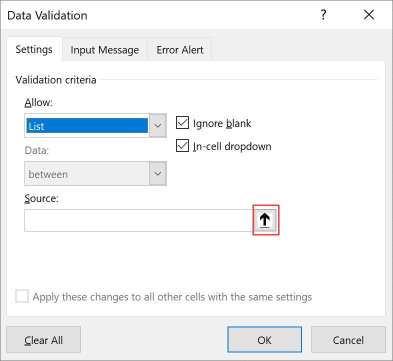
Select the cell where the Dependent list will go. In this example, I have selected the cell under Expense Type heading.

Under the Data tab, in the Data Tools group, click Data Validation.

Under the Allow drop-down, select List.

For the Source, enter =indirect(B2). B2 refers to the cell of the Parent list, for example, the cell under the Expense Category. The Indirect Function will use this as a reference point to drive the sub list options.

Alternatively, if the options in the Parent list have spaces, for example, Business Travel, then you will need to use this formula instead =indirect(Substitute(B2, “ “, “_”))

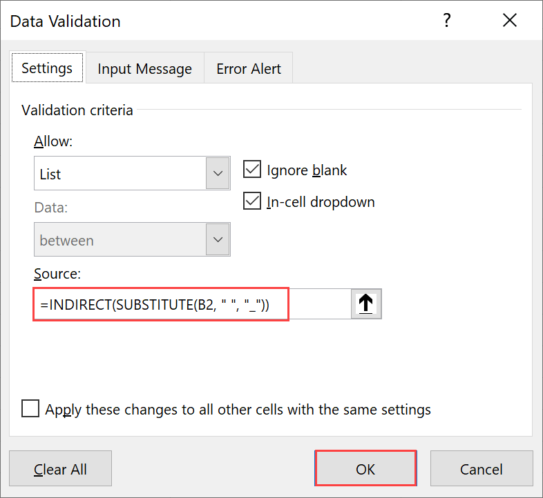
The above Substitute function will reverse this by replacing the underscore with a space.

Click OK to complete.

Test your Dependent Drop-Down list.

Watch these!

You've read the guide now watch the videos that show you how. There is a nice little challenge at the end of each video.

Need help?

Do you need help with something that you're working on? Maybe you're looking for a quicker way to do something or is there something that you struggle with? Pop an email to Suggestions@ReadySteadyXL.com - I will find the solution for you and cover it in one of my guides or videos.